2. Definitions
2.1. Symbols definitions
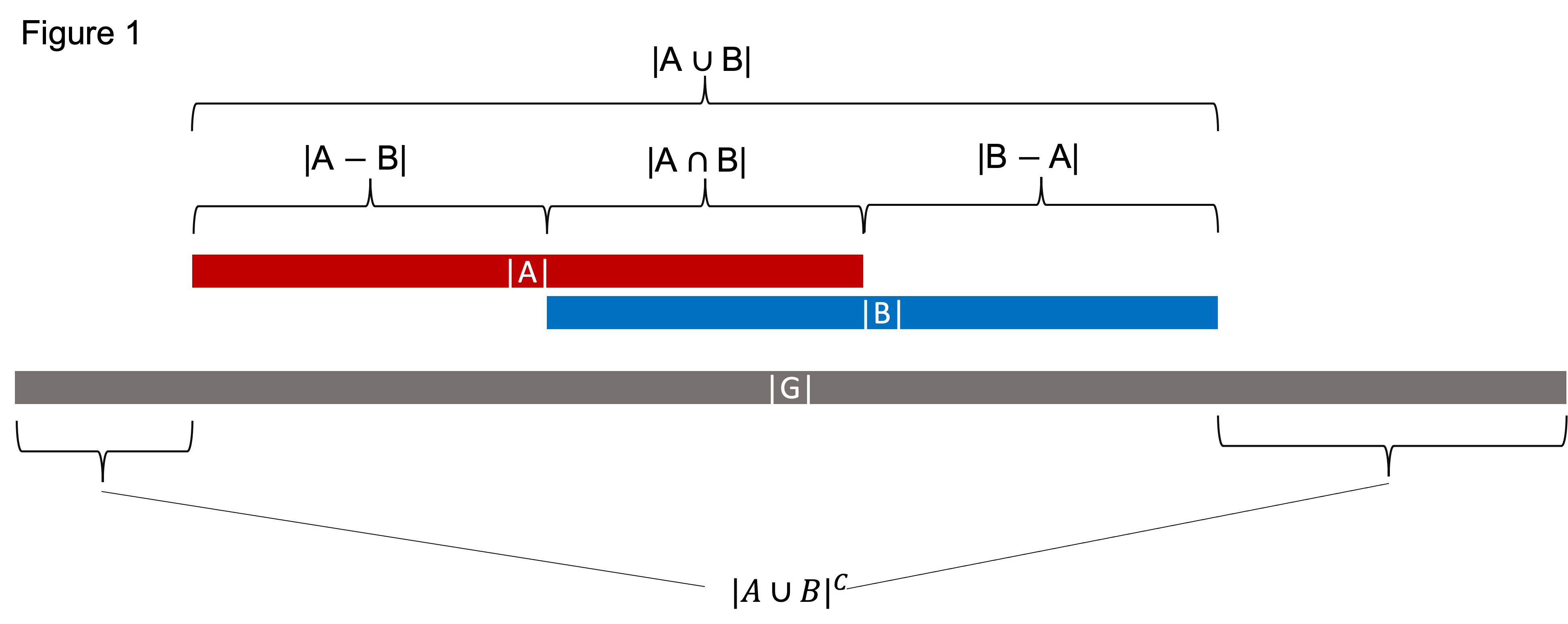
We have two sets of genomic intervals A and B, and the genomic background is G. In Figure 1 below, both A and B contain only one genomic region for the purpose of clarity, but the definitions are still applicable if A and B have many intervals.
Symbols are defined as:
- |A|
The cardinality of A (i.e., all the non-redundant bases covered by A). For example, if A contains two genomic intervals: “chr1 0 10”, “chr1 5 15”, then |A| = 15.
- |B|
The cardinality of B (i.e., all the non-redundant bases covered by B).
- |G|
The genomic background. Depending on the context, this can be the whole genome, all the cis-regulatory elements, all the promoters, all the TF binding sites in the genome, etc. A and B must be the subsets of G.
- |A ∪ B|
Union of A and B (i.e., bases covered by A or B).
- |A ∩ B|
Intersection of A and B (i.e., bases covered by A and B simultaneously). This is commonly used to measure the collocation of A and B.
- |A − B|
Difference (A not B) (i.e., bases covered by only A but not B).
- |B − A|
Difference (B not A) (i.e., bases covered by only B but not A).
- |A ∪ B|^𝐶
Complement of |A ∪ B| (i.e., bases NOT covered by A or B).
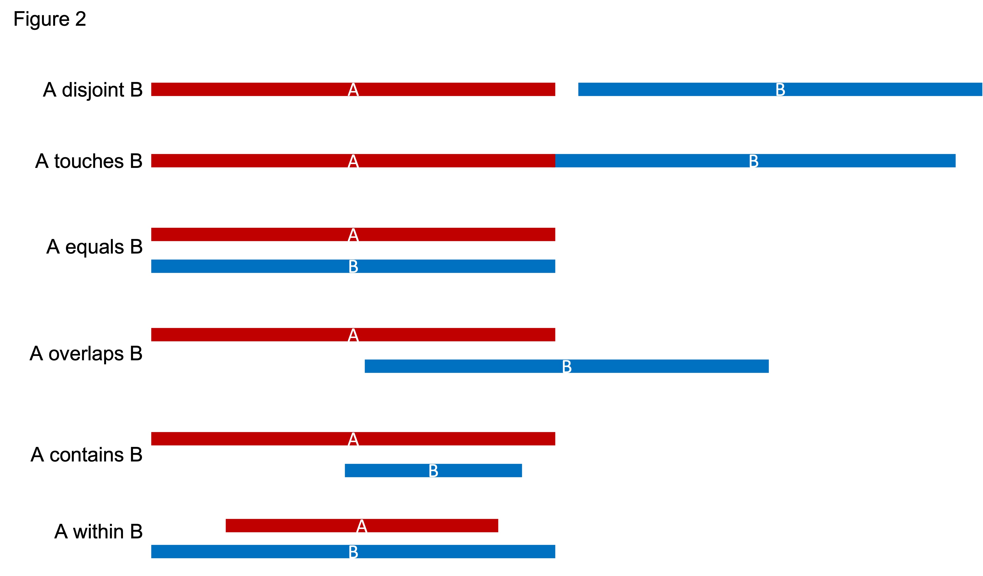
2.2. Spacial Relations of Genomic regions (SROG)
There are six different spacial relations between two genomic regions (A and B). As illustrated below:
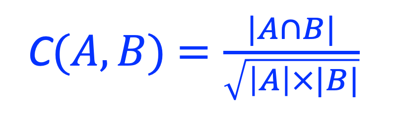
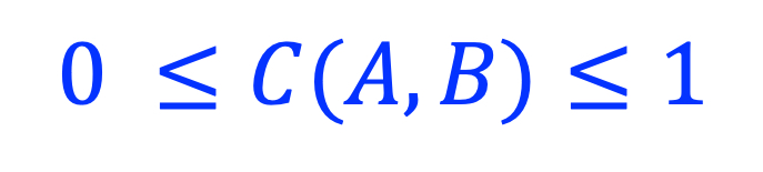
2.3. Collocation coefficient (C)
The collocation coefficient between A and B is calculated as the ratio between |A ∩ B| and the geometric mean of |A| and |B|. C(A,B) is a value between [0, 1], with 0 indicating ‘no overlap’, and 1 indicating ‘100% overlap’ (i.e., A and B are identical). C(A, B) is defined as 0 when |A| = 0 or |B| = 0, or |A| = |B| = 0.
- Overall collocation coefficient
The collocation coefficient between two sets of genomic regions. For example, you can use the overall collocation coefficient to measure the cobindability of two transcription factors.
- peakwise collocation coefficient
The collocation coefficient between two genomic intervals (A protein-bound genomic region is called “peak” in ChIP-seq experiment).
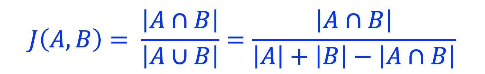
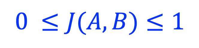
2.4. Jaccard coefficient (J)
The Jaccard similarity coefficient, also known as the Jaccard index. It is the ratio between intersection and union. J(A, B) is defined as 0 when |A| = 0 or |B| = 0, or |A| = |B| = 0.
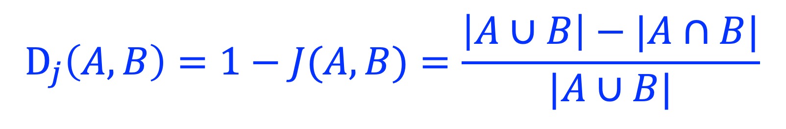
The Jaccard distance Dj is calculated as:
Similar to O(A,B), we have an overall Jaccard coefficient and peakwise Jaccard coefficient.
Note
The Jaccard coefficient implemented here is slightly different from BEDTools jaccard function.
When calculating the union, BEDTools only use the intervals that are overlapped with each other, while we use all the intervals.
- overall Jaccard coefficient
The Jaccard coefficient between two sets of genomic regions.
- peakwise Jaccard coefficient
The Jaccard coefficient between two genomic intervals.
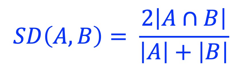
2.5. Sørensen–Dice coefficient (SD)
Sørensen–Dice coefficient, also called Sørensen–Dice index, Sørensen index or Dice’s coefficient. SD(A, B) is defined as 0 when |A| = 0 or |B| = 0, or |A| = |B| = 0.
Jaccard coefficient (J) can be converted into Sørensen–Dice coefficient (SD) and vice versa:
J = SD/(2-SD) and SD = 2J/(1+J)
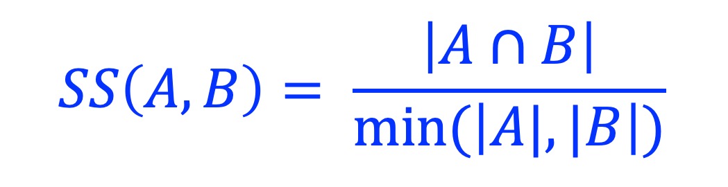
2.6. Szymkiewicz–Simpson coefficient (SS)
Szymkiewicz–Simpson coefficient is defined as the size of the intersection divided by the smaller size of the two sets.
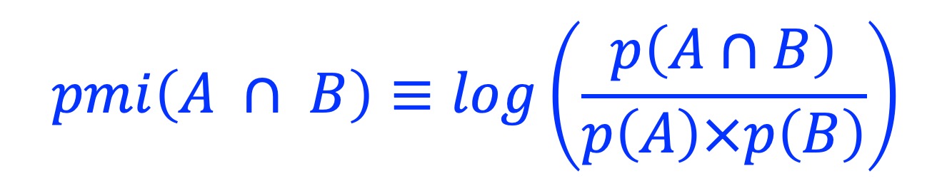
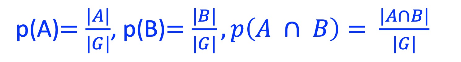
2.7. Pointwise mutual information (PMI)
Pointwise mutual information (PMI) is one of the standard association measures in collocation analysis. It measures how much the observed overlaps differ from what we would expect them to be. Assume A and B represent two sets of genomic regions bound by transcription factors A and B; respectively, PMI measures if A and B bind together or separately.
PMI is calculated as:
where
- PMI = 0
Indicates that A and B are independent.
- PMI > 0
Indicates that the overlapping between A and B is in a frequency higher than what we would expect if A and B are independent (i.e, A and B tend to bind together).
- PMI < 0
Indicates that the overlapping between A and B is in frequency lower than what we would expect if A and B were independent. (i.e., A and B tend to bind separately).
Note, PMI has no boundaries:

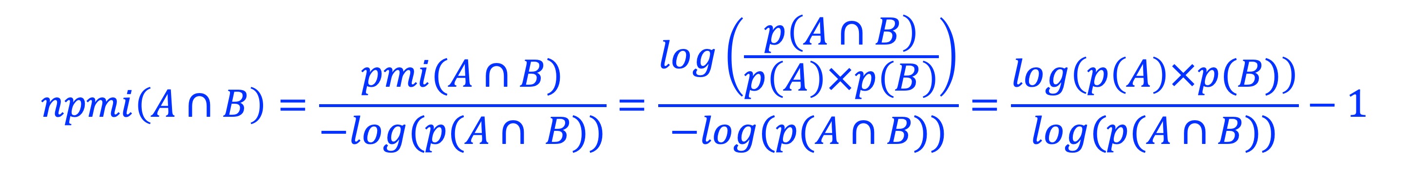
2.8. Normalized pointwise mutual information (NPMI)
Normalized pointwise mutual information (NPMI) is calculated as:
Note, after normalization, NPMI is confined to [-1, 1]:
2.9. Which metric to use?
Use the Z-score approach to combine all the six metrics as an overall measure, or choose the Collocation coefficient (C) and NPMI which generally performs better than other approaches.